
Before a computer could flag a suspicious area in a scan, it had to treat anatomy as measurable data. In the earliest digital medical images, a pixel was more than a point on a display: it represented an X-ray attenuation value, a radiofrequency-derived signal, or an ultrasound echo. Much of the field’s early work addressed a basic question: how could imperfect measurements be turned into images whose structures could be compared, separated, and quantified?
Medical image analysis emerged at the intersection of radiology, nuclear medicine, signal processing, statistics, computer science, and engineering. Its history is not one of automation simply displacing human interpretation. The aim was usually more modest and more useful: make images reproducible, expose subtle patterns, and convert visual observations into measurements that could support research and clinical decisions.
Digital images arrive in medicine
Conventional radiography had demonstrated the clinical value of imaging long before digital analysis. The major change came with modalities built around computation. X-ray computed tomography, introduced clinically in the 1970s, reconstructs cross-sectional anatomy from many measured projections. Each reconstructed slice is a matrix of numerical values, often expressed on the Hounsfield scale, where air, water, fat, and dense bone fall within characteristic ranges.
That numerical basis changed the questions researchers could ask. Rather than inspecting film alone, they could calculate intensity histograms, measure an organ’s area, estimate a lesion’s volume, or compare regions over time. Magnetic resonance imaging introduced rich contrast related to tissue properties and acquisition settings. Positron emission tomography and related nuclear-medicine methods supplied functional signals, often at lower spatial resolution but with direct relevance to metabolism or receptor activity. Ultrasound provided real-time imaging, while bringing difficult speckle noise and variable appearances.
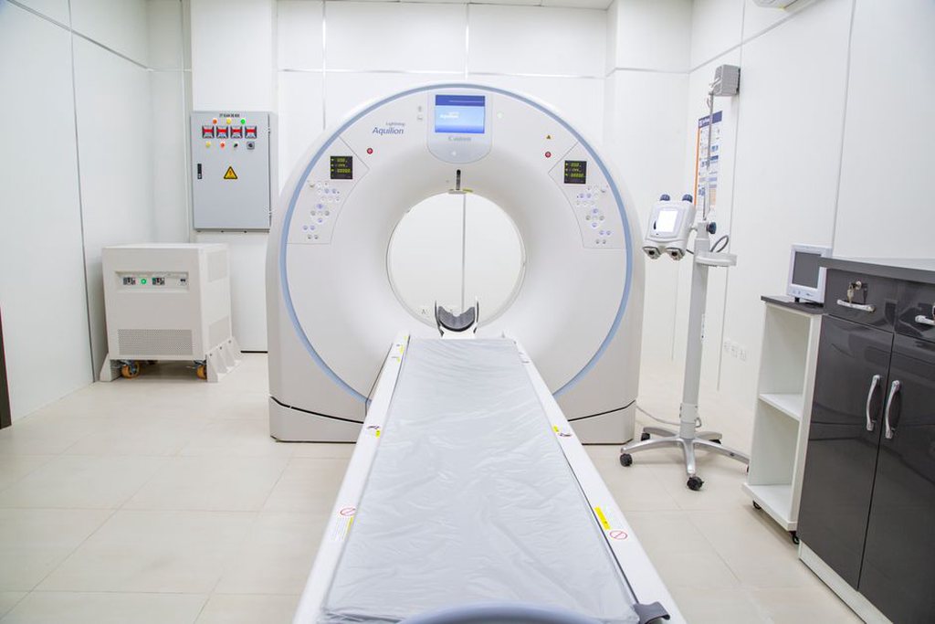
None of these modalities produced uniformly clean data. Noise, limited resolution, motion, reconstruction artifacts, scanner differences, and changing acquisition protocols all affected the image. Early analysis was therefore inseparable from image processing: the signal often had to be improved or standardized before researchers could identify anatomy or disease.
From enhancement to measurable structure
Filtering, contrast, and edges
Many first-generation methods came directly from digital signal processing. Smoothing filters reduced high-frequency noise, but too much smoothing could erase small vessels or lesion boundaries. Sharpening and edge-enhancement filters made tissue transitions easier to see, while also risking greater noise. Histogram equalization and window-level adjustments improved the display of selected intensity ranges. Radiologists still use this principle: a CT scan displayed for fine lung detail looks different from one displayed for soft tissue.
Edge detection offered an obvious route to delineating structures. Gradient-based operators locate abrupt intensity changes, while second-derivative methods emphasize ridge-like and boundary-like features. Their limits became clear in medical images, where anatomical borders may be weak, interrupted, or blurred by partial-volume effects. A single voxel can represent a mixture of tissues, particularly in thick slices or low-resolution scans. An edge map alone was therefore rarely enough to define a dependable organ contour.
Segmentation: assigning pixels to anatomical regions
Segmentation—the division of an image into meaningful regions—became one of the central tasks in medical image analysis. Thresholding was among the simplest methods. When a tissue occupied a distinct intensity interval, values within that range could be selected; CT bone extraction is a familiar example. Fixed thresholds break down, however, when intensities overlap, contrast changes, or pathology alters the expected appearance.
Researchers expanded on thresholding with region growing, in which neighboring pixels similar to a seed point are added to a region. Morphological operations, based on local shape and connectivity, could fill holes, remove isolated artifacts, or separate touching objects. Connected-component analysis then helped a system choose a plausible anatomical candidate according to size, location, or shape.
Later classical methods stated their assumptions more clearly. Active contours, often called snakes, moved a curve toward image boundaries while imposing smoothness. Level-set methods represented a moving boundary implicitly and handled splits or merges more naturally. Markov random fields and graph-based methods combined local image evidence with a preference for spatially coherent labels. These techniques did not understand anatomy as a clinician does; they encoded useful assumptions about continuity, intensity, and expected form.
- Pixel-level evidence captures intensity, texture, gradients, or local filter responses.
- Spatial context reflects the fact that neighboring tissue labels are usually related.
- Prior knowledge restricts results according to expected anatomy, shape, or position.
- Human review remains essential when boundaries are ambiguous or clinically consequential.
Registration: making images correspond
A second foundational task is registration: aligning two or more images so that corresponding locations refer to the same anatomy. Registration supports comparisons over time, modality fusion, surgical planning, and the construction of population atlases. In a longitudinal brain study, for example, an apparent intensity change is hard to interpret if head position differs between scans.
Early registration often relied on rigid transformations—translations and rotations—suited to relatively fixed structures such as the skull. Affine transformations added scaling and shear. Soft tissue, however, changes with breathing, posture, organ filling, growth, and disease. Non-rigid registration introduced deformation fields to model such local changes, generally with regularization that penalized implausibly jagged warps.
Multimodal registration introduced a separate difficulty: a bright region in one modality may not be bright in another. Mutual-information methods became influential because they measure statistical dependence between intensity distributions rather than requiring intensities to match directly. Their success reflects a recurring pattern in the field: familiar computer-vision methods often had to be recast around the physics and meaning of particular imaging modalities.
Feature extraction and computer-aided diagnosis
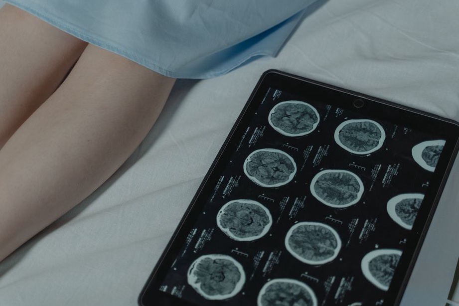
Once regions could be located or aligned, researchers looked for features that distinguished normal tissue from abnormal tissue. These included size, compactness, boundary irregularity, intensity statistics, texture descriptors, symmetry, and change over time. In mammography, systems examined microcalcification clusters and mass characteristics. In chest imaging, they searched for candidate nodules. In brain imaging, they measured lesion burden or regional volume.
This work is often described as computer-aided detection or computer-aided diagnosis, and the distinction matters. Detection systems flag candidates for inspection. Diagnostic systems estimate whether a finding belongs to a disease category. Historically, many were intended as second readers, offering marks or scores to assist clinicians rather than replace them.
During the 1990s and 2000s, classifiers commonly depended on engineered features and statistical learning: linear discriminants, k-nearest-neighbor methods, decision trees, support vector machines, modest neural networks, and ensemble methods. Their results depended heavily on segmentation quality and feature design. A classifier cannot restore information lost when a lesion is cropped incorrectly or represented by unstable measurements.
Why validation became a technical issue
Medical images are not independent snapshots drawn from a generic visual dataset. Multiple slices may come from one person, scans from one hospital may share protocol-specific traits, and disease prevalence differs between populations. If images from the same patient appear in both training and test data, reported performance can be unrealistically optimistic. A model may also learn scanner markings or acquisition differences rather than pathology, appearing accurate in one dataset before failing elsewhere.
Evaluation practices therefore focused on carefully separated patient cohorts, independent test sets, sensitivity and specificity, receiver operating characteristic curves, and observer studies. For segmentation, overlap measures such as the Dice coefficient became common. Even a high overlap score can conceal an error along a clinically important boundary. Ground truth is complicated as well: experts may disagree, and pathology or follow-up may not be available for every case.
| Task | Typical early technique | Persistent limitation |
|---|---|---|
| Enhancement | Filtering and contrast transformation | Noise reduction can remove detail |
| Segmentation | Thresholding, region growing, active contours | Weak or variable tissue boundaries |
| Registration | Rigid, affine, and deformable transforms | Real anatomy may change non-uniformly |
| Classification | Handcrafted features with statistical classifiers | Dataset bias and limited generalization |
The bridge to contemporary learning methods
Modern deep learning shifted the balance between hand-designed features and learned representations, particularly as larger annotated datasets and stronger hardware became available. Convolutional neural networks could learn useful image features from examples, while encoder-decoder architectures made pixel-wise segmentation feasible at scale. The older problems did not disappear: registration remains important, acquisition variation still affects results, labels still contain uncertainty, and clinical deployment still demands careful validation.
The continuity becomes apparent when a modern segmentation system is examined closely. Its inputs may be normalized to reduce scanner-related variation; specialists may produce labels according to a stated protocol; outputs may be checked for anatomical plausibility; and accuracy may be reported separately by site, scanner, demographic group, and disease subtype. These practices grew out of earlier work on measurement, spatial constraints, and fair evaluation.
When reading a historical paper—or judging a newer imaging claim—the most revealing technical detail is often the reference standard. Were contours supplied by one expert, a consensus panel, pathology, longitudinal follow-up, or an algorithmic proxy? The answer defines what the reported system was actually trained to reproduce.