
Before deep learning, a medical image system rarely began by deciding what diagnosis a scan contained. It usually faced a narrower question first: where is the organ, lesion, vessel, or boundary? A CT volume can contain thousands of anatomical structures and acquisition artifacts. An X-ray overlays ribs, lung texture, and soft tissue. In ultrasound, speckle may dominate the frame. Before assigning a label, researchers had to derive a usable representation from imperfect pixels.
That order shaped the field for decades. Medical image analysis brought together image processing, geometry, statistics, anatomical knowledge, and clinical measurement. Systems were often built for tightly defined tasks: outlining the left ventricle, counting cell nuclei, registering serial brain scans, identifying microcalcifications, or estimating tumor volume. Their strengths and limitations followed directly from those design choices.
From image formation to measurable structures
Medical images are measurements, not ordinary photographs. Their appearance reflects a physical acquisition process: X-ray attenuation in radiography and CT, proton relaxation in MRI, reflected sound in ultrasound, or tracer distribution in nuclear medicine. Each modality comes with its own combination of useful contrast, noise, artifacts, and spatial scale.
Algorithms could therefore make use of modality-specific assumptions. In CT, voxel values are calibrated in Hounsfield units, so simple intensity thresholds can be useful for certain tasks. Air-filled lungs, dense bone, and many soft tissues fall into distinct broad ranges. MRI provides strong soft-tissue contrast but has no universal intensity scale: the same tissue may appear quite different across scanners, pulse sequences, and sites. Ultrasound supports real-time imaging, yet speckle and shadowing can hide genuine boundaries and complicate segmentation.
Researchers commonly divided a pipeline into several stages:
- Acquisition and quality control: inspect resolution, field of view, artifacts, and missing slices.
- Preprocessing: reduce noise, normalize intensities, correct bias fields, or enhance contrast.
- Localization: limit analysis to an anatomical region or plausible search area.
- Segmentation or feature extraction: identify structures and calculate descriptors.
- Modeling and decision support: estimate a measurement, detect a suspicious finding, or assign a statistical score.
- Evaluation: compare results with expert annotations, pathology, follow-up, or another accepted reference standard.
Any stage could fail on its own. A sophisticated classifier could not recover reliable evidence after a registration error, a misplaced region of interest, or a poorly defined ground-truth contour.
Segmentation: the central technical challenge
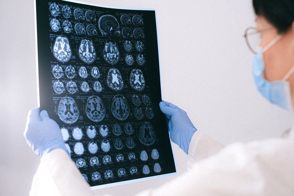
Segmentation assigns pixels or voxels to structures of interest. The idea is straightforward when an organ is clearly visible, but anatomical boundaries are often ambiguous. A tumor may blend into neighboring tissue, partial-volume effects may mix tissue types within a voxel, motion can blur an edge, and disease may alter the shape an algorithm expects.
Thresholds, regions, and edges
Thresholding was one of the most direct approaches. If a target occupied a known intensity range, voxels in that range could be selected. CT bone extraction was a classic favorable case. Thresholds alone, however, often merged separate structures or excluded legitimate low-contrast tissue. Researchers added connected-component analysis, morphological opening and closing, hole filling, and anatomical constraints to turn a raw binary mask into a plausible anatomical structure.
Region-growing methods expanded from a seed point when neighboring pixels met a similarity condition. They could work well for compact areas with relatively consistent intensity, but the choice of seed and stopping rule mattered. Leakage into adjacent tissue remained a persistent problem, especially where boundaries were weak.
Edge-based methods looked for abrupt changes in image values, often through gradients. The appeal was obvious: a boundary should produce an edge. Medical images complicated that assumption. Noise creates false edges, while real tissue transitions can be gradual. Smoothing can suppress noise, but it may also erase fine structures. In practice, systems often combined edge evidence with region statistics instead of relying on either alone.
Deformable models and anatomical priors
Active contours, or “snakes,” and later level-set methods described a boundary that moved under competing forces. Image-derived forces pulled the contour toward edges or homogeneous regions, while smoothness terms discouraged implausibly jagged shapes. Level sets were useful when a boundary could split or merge during optimization, as in some vascular and lesion-segmentation problems.
Statistical shape models took another approach. Built from manually annotated examples, they described ordinary variation in an anatomical structure while constraining results to shapes observed in a training population. Active shape and active appearance models became influential in work on facial landmarks, bones, and cardiac anatomy. Their limitation was just as important: unusual anatomy, severe disease, incomplete coverage, or a population unlike the training set could make a valid structure seem “implausible” to the model.
Features made clinical questions computable
Before end-to-end neural networks, a system’s input was often a hand-engineered feature vector. Researchers selected measurements meant to capture clinically relevant properties: size, shape, intensity distribution, texture, symmetry, spatial position, or change over time.
| Feature family | Typical measurements | Common use |
|---|---|---|
| Intensity | Mean, variance, histogram percentiles | Tissue characterization and lesion contrast |
| Shape | Area, volume, compactness, curvature, eccentricity | Organ measurement and mass characterization |
| Texture | Co-occurrence statistics, run lengths, filter responses | Characterizing tissue patterns and radiographic texture |
| Spatial relations | Distance to landmarks, relative position, symmetry | Reducing false detections through anatomy |
| Temporal features | Motion, enhancement curves, serial-volume change | Cardiac imaging and longitudinal monitoring |
Texture analysis shows both the appeal and the fragility of this approach. A lesion may have internal variation that average intensity cannot capture, so studies used gray-level co-occurrence matrices, Gabor filters, wavelets, and local binary patterns to quantify it. Those measurements could be sensitive to reconstruction settings, scanner protocols, pixel spacing, and the segmentation used to define the region. An association reported at one hospital could weaken sharply on images from another scanner or site.
Feature selection was therefore a major concern. Small clinical datasets could yield dozens or hundreds of descriptors from relatively few patients. Selecting features after inspecting the same data used for evaluation could produce overly optimistic results. Cross-validation helped only when feature selection, parameter tuning, and preprocessing were repeated within each training fold, rather than completed once on the full dataset.
Classifiers were only one component
After features were extracted, researchers used statistical classifiers including linear discriminant analysis, logistic regression, k-nearest neighbors, decision trees, random forests, support vector machines, and Gaussian mixture models. These were not merely primitive predecessors to neural networks. Many were mathematically strong and appropriate for small datasets. Their performance depended heavily on whether the selected features contained stable evidence for the decision at hand.
Support vector machines were especially common in the 2000s because they could work effectively in high-dimensional feature spaces and offered kernel functions for nonlinear decision boundaries. Still, a high score on a carefully selected dataset did not necessarily indicate clinical value. Image-level accuracy could conceal poor sensitivity for subtle lesions. A balanced research sample might bear little resemblance to disease prevalence in routine care. A classifier trained on images from one scanner might learn site-specific appearance rather than pathology.
Computer-aided detection (CADe) and computer-aided diagnosis (CADx) made the difference clear. A CADe system marked potentially suspicious regions for review, whereas CADx aimed to characterize a finding or estimate its likelihood of belonging to a diagnostic category. In both cases, the intended role was generally assistance rather than autonomous diagnosis. False positives carried a practical cost: every extra mark could consume a clinician’s attention and weaken confidence in the tool.
Registration connected images across space and time
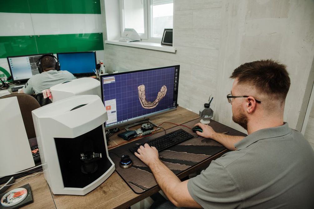
Registration estimates the transformation that aligns one image with another. It supported comparisons between pre- and post-treatment scans, fusion of CT with MRI or PET, atlas-based labeling, and correction for patient repositioning. Rigid registration modeled translation and rotation. Affine registration added scaling and shear. Deformable registration accommodated local anatomical variation.
The difficulty was that an alignment could look convincing while being wrong in a clinically important area. Similarity measures such as mutual information made multimodal registration possible by comparing statistical dependence rather than identical intensities. Deformable methods added smoothness regularization so neighboring locations would not move arbitrarily. Even so, a mathematically smooth deformation was not necessarily physiologically plausible, particularly around tumors, surgical changes, or organs altered by breathing and filling.
Registration also reveals a defining feature of pre-deep-learning research: its assumptions were usually explicit. A paper could state its transformation family, similarity metric, interpolation scheme, regularization weight, and landmark error. That level of detail made it easier to see why an approach worked on brain MRI but struggled with abdominal CT.
Evaluation required more than a single accuracy number
Medical-image studies had to separate technical agreement from clinical validity. For segmentation, overlap measures such as the Dice similarity coefficient and Jaccard index were common, though they could hide boundary errors in small structures. Mean surface distance, Hausdorff distance, volume error, and repeatability offered other useful views. For detection and classification, sensitivity, specificity, receiver operating characteristic curves, area under the curve, precision, and false positives per image answered different questions.
Reference standards were not always definitive. Expert readers can disagree, particularly over weak boundaries or early disease. Pathology may be available only for selected cases. Follow-up can establish an outcome without providing a precise lesion contour. Good studies reported who labeled the data, whether readers were blinded, how disagreements were resolved, and whether test cases were held out by patient rather than merely by image slice.
That final distinction matters greatly for 3D scans. If adjacent slices from one patient appear in both training and test sets, their similarity can inflate performance. A more credible split keeps every image from a patient in the same partition. External testing at another institution is stronger still because it exposes vulnerability to differences in population, scanner hardware, protocols, and reporting practice.
Why these methods remain historically and practically important
Deep learning changed medical imaging by learning layered representations from large datasets, but it did not remove older problems involving acquisition, labels, validation, calibration, workflow, and interpretability. Current systems still rely on registration, morphology, image normalization, geometric constraints, and carefully defined clinical endpoints. They also inherit a central lesson of earlier work: a technically impressive model may fail outside the setting that produced its training data.
Pre-deep-learning systems also left behind a valuable engineering discipline. Their intermediate outputs—an organ mask, vessel centerline, detected candidate, shape coefficient, or registration field—could be inspected by domain experts. That made errors visible in ways an opaque final score often does not. The broader pattern-recognition environment of the period appears in the 2013 PRASA proceedings document discussed in “The 2013 PRASA Proceedings: Decoding ‘proceedings 2013 prasa2013 02 pdf’”, where applied methods were commonly presented through explicitly defined representations and evaluations.
When reconstructing a historical paper or archived prototype, begin with the imaging modality, patient-selection criteria, unit of analysis, annotation protocol, preprocessing steps, and patient-level data split. Only then is it useful to compare reported classifier performance with another study. An area under the curve of 0.90 says little without knowing whether it came from 40 lesions on one scanner or an independent cohort acquired under a different protocol.