
A computer can flag a suspicious patch on a mammogram without knowing whether the patient has cancer. That distinction shaped the move toward machine learning in medical diagnostics. Researchers trained systems to recognize patterns in images, measurements, and records, while clinicians had to interpret those patterns alongside symptoms, history, and test results. Software did not suddenly replace diagnosis; learned statistical judgments entered tasks once handled by fixed thresholds, visual inspection, or hand-written rules.
From rules to learned boundaries
Earlier diagnostic software often encoded expert knowledge directly. A rule might flag a laboratory value above a set threshold, or an image-processing pipeline might mark objects with a particular brightness and shape. Such methods remained useful, but biological variation resisted exhaustive rules. A small lesion could resemble normal tissue; noise could obscure an abnormal heartbeat; and the significance of one measurement could depend on several others.
Machine learning took a different approach. Investigators assembled examples with known labels or outcomes, extracted measurable features, and fitted a model to separate categories or estimate risk. A classifier could learn that several weak clues together were more informative than a single cutoff. This extended statistical pattern recognition rather than breaking with it. Logistic regression and discriminant analysis had long been relevant to clinical prediction; during the 1990s and 2000s, researchers also investigated neural networks, decision trees, support vector machines, and ensemble methods.
The distinction between detecting a finding and diagnosing a patient remained essential. A model might locate possible pulmonary nodules on a chest image, but determining their cause required clinical context and often follow-up. A model trained to predict a recorded diagnosis might also learn how a hospital orders tests or documents cases, rather than learning only about the underlying disease.
Why images became an early testing ground
Radiology, pathology, and ophthalmology produced data with visible structures that researchers could annotate and compare. Computer-aided detection for mammography was a prominent early example: software highlighted regions for a radiologist to inspect. A mark was not a verdict. False alerts could lengthen reading time or prompt unnecessary investigation, while missed findings limited the system’s value.
In a typical mid-2000s image-analysis project, researchers corrected acquisition artifacts or standardized contrast, then identified a region of interest. They measured texture, intensity, boundary shape, or symmetry before passing those features to a classifier. Training determined how to weight the measurements, but people still chose much of the representation. Segmentation—separating an organ, vessel, or lesion from surrounding tissue—was often as difficult as classification. If the boundary was wrong, even a well-trained classifier received misleading measurements.
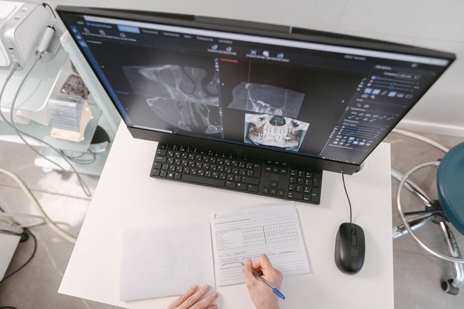
For background on the earlier work of converting scans into quantitative measurements, see Medical Image Analysis in the Early 2000s: From Scans to Measurements.
Imaging exposed another persistent problem: a model could recognize acquisition conditions instead of disease. Scanner settings, image compression, hospital-specific labels, and marker positions might correlate with diagnoses in a training set. Results from randomly divided images at one institution could therefore overstate performance elsewhere. A more demanding evaluation separated patients—and, ideally, institutions or time periods—between development and testing.
What changed beyond the scan
Medical diagnostics involves more than images. Laboratory values, vital signs, electrocardiograms, and clinical records contain patterns that may be hard to combine mentally across many cases. Learning-based systems could estimate the likelihood of a condition from multiple inputs or help prioritize results for review. Each source also brought failure modes: missing tests, inconsistent units, changes in coding practice, and measurements taken precisely because a clinician already suspected a disease.
The label is part of the experiment
Supervised learning needs a target. Researchers might use a pathology result, an expert annotation, a discharge diagnosis, or an outcome recorded months later. These targets are not interchangeable. A pathology-confirmed label may be precise but available only for selected patients. A billing code covers more people but can reflect administrative practice. Expert readers may disagree about an image finding, especially near a diagnostic boundary.
Consider a model trained to identify infection from hospital records. If its label depends partly on whether antibiotics were prescribed, it may learn prescribing patterns rather than infection itself. That could still help predict treatment decisions, but it would not make the model an independent disease detector. How researchers constructed the label matters as much as which model they chose.
Neural networks before and after deep learning
Neural networks were studied in medicine well before modern deep learning. Earlier networks commonly used features selected by researchers because datasets and computing power limited what could be learned directly from pixels. Later, deep convolutional networks made it practical to learn image representations from large collections of examples, reducing the need to specify every visual feature by hand. Preprocessing, annotation, and clinical validation still mattered. More decisions about representation had moved into training, where they could be harder to inspect.
Accuracy depends on the clinical task
A single accuracy percentage rarely tells a clinician whether a model will be useful. Suppose a system screens 10,000 people for a condition present in 1% of them. At 90% sensitivity, it finds 90 of the 100 affected people and misses 10. At 90% specificity, it also flags 990 of the 9,900 unaffected people. Of 1,080 positive alerts, only 90 correspond to affected people—about 8%. That does not make the system worthless; it shows why prevalence and the cost of follow-up matter.
- Sensitivity measures how many affected cases are found. It matters when missed cases are especially harmful.
- Specificity measures how many unaffected cases are correctly left unflagged. It matters when false alerts create burdens or risks.
- Calibration asks whether predicted probabilities match observed frequencies. A score of 20% should correspond to roughly two cases in ten among comparable patients.
- Clinical impact asks what changes when a result enters the workflow: timing, decisions, follow-up tests, and patient outcomes.
Area under the receiver operating characteristic curve summarizes how well a model ranks cases across thresholds, but it does not select the right threshold for a clinic. A triage tool designed to avoid missing urgent cases may tolerate many false alerts. A system that recommends an invasive procedure needs a different trade-off, examined closely. Evaluation must account for the existing decision process and the people using the tool, not just an abstract benchmark.
Why promising studies did not always translate
Small, carefully selected datasets let researchers test ideas, but they could conceal the diversity of routine care. Cases and controls drawn from separate sources might be easier to distinguish than patients arriving consecutively at a clinic. If images from the same patient appeared in both training and evaluation, a model might seem to generalize while recognizing patient-specific features. Even an independent held-out test set could gradually become part of development if researchers repeatedly experimented against it.
Prospective testing posed a different question: how would a fixed system behave on new patients under ordinary working conditions? A report needed to say whether it excluded poor-quality scans, whether patients with missing records received predictions, and how often clinicians disagreed with a flag. Subgroup analysis could expose uneven performance across patient populations or equipment types, though small subgroup samples left those estimates uncertain.
Deployment could change the meaning of an output, too. An alert that helped a specialist spot a subtle finding might distract a generalist facing a long queue of false positives. A probability displayed without a clear time horizon or target outcome could be mistaken for a diagnosis. Human review alone was no guarantee of independent judgment if reviewers grew accustomed to accepting automated suggestions; interface design and workflow mattered.
Reading the historical shift precisely
Mid-2000s research papers often followed a recognizable pipeline: acquire data, preprocess it, extract features, train a classifier, and report test-set results. Later deep-learning studies changed the technical center of that pipeline, but familiar questions remained. What counted as a case? Who supplied the reference label? Were training and test patients separate? Could the method handle another clinic’s images or records?
Those answers separated a pattern-recognition demonstration from evidence for clinical use. Progress could be incremental: handling an unfamiliar scanner or a previously excluded low-quality image might matter more in practice than a small improvement on a selected test set. When assessing a reported accuracy figure, check who entered the test cohort. Were all consecutive scans included, or only those with a confirmed result? That eligibility rule may tell you more about the claim than the headline number.