
In 2005, the typical consumer webcam captured video at 30 frames per second — barely enough for casual motion, but a blurry nightmare for tracking a fast-moving tennis ball or a pedestrian stepping into a crosswalk. Inside academic computer vision labs, however, the standard was already double that, and often quadruple. The number 120 — 120 fps — became a quiet benchmark for a generation of tracking, stereoreconstruction, and motion analysis research. It was not an arbitrary round figure; it emerged from engineering constraints, sensor availability, and the need for temporal oversampling that would later underpin modern high-speed vision systems.
The earliest high-speed cameras used in vision research were adapted from industrial machine vision. By the early 2000s, CMOS sensors capable of global shutter and 120 fps at VGA resolution (640×480) were becoming affordable for university labs. Basler, Point Grey (later FLIR), and Mikrotron offered cameras that could sustain 120 fps over FireWire or Camera Link. The number 120 was a sweet spot: it matched the old NTSC field rate (59.94 Hz doubled) and fell exactly at 4× the standard 30 fps, making temporal interpolation algebraically neat. PAL regions used 100 fps sometimes, but 120 became de facto in North American and Japanese labs.
Why 120 Fps Mattered for Tracking Algorithms
Early object trackers — mean-shift, Kalman filter-based, and the nascent particle filters — all suffered from two fundamental problems: target aliasing and motion blur. At 30 fps, a car moving at 60 km/h travels roughly 0.55 meters between frames (assuming a 10 m field of view). At 120 fps, that displacement shrinks to 14 cm. The smaller inter-frame motion allowed trackers to rely on simple linear motion models without drifting. The covariance matrices in Kalman filters could be tighter, and particle filters required fewer particles to maintain a plausible distribution.
One of the earliest systematic studies of frame-rate effects on tracking came from the Computer Vision Laboratory at the University of Maryland, where in 2004 a team ran comparative experiments on a dataset of high-speed hand gestures. They varied the frame rate from 15 to 120 fps by subsampling the same 240 fps source video. The result: a sharp knee in tracking accuracy improvement up to 120 fps, after which gains were marginal. The paper, presented at CVPR 2005, argued that for human-scale motions, 120 fps was the optimal trade-off between data rate and performance. The number 120 thus became a recommended parameter in many subsequent tracker benchmark.
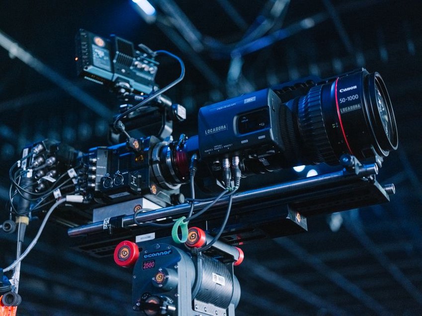
Stereoreconstruction at 120 Hz
Stereo vision researchers also benefited. Wide-baseline stereo matching relies on consistent pixel correspondences across two cameras. When both cameras run at 120 fps and are hardware-synchronized, the temporal synchrony error drops below 0.5 ms — negligible for most scenes. This allowed dense disparity maps without motion artifacts for scenes with moving objects. At the 2005 International Workshop on Stereo and Multi-Baseline Vision, a group from Tōkyō Institute of Technology demonstrated a real-time stereo system producing 320×240 disparity maps at 120 fps using a pair of Point Grey Flea cameras. They used sum of absolute differences on GPU-accelerated hardware (then still unusual). The 120 fps rates made it possible to track hand gestures in 3D with subcentimeter accuracy.
The 120 fps Dataset Legacy
Several important datasets from that era were recorded at 120 fps. The VIVID (Vision and Image Understanding) dataset for action recognition included sequences at 120 fps, though most research used downsampled versions. The KTH actions dataset (2004) was recorded at 25 fps, but the later Weizmann dataset had some 50 fps clips. The 120 fps datasets were mostly created in-house: e.g., the University of Oxford's 'Billiards' sequence (used in the seminal 'Video Textures' paper) was shot at 120 fps to capture the ball's spin. These datasets became testbeds for motion debluring algorithms as well.
Limitations: Storage and Processing
The downside was obvious: one minute of 640×480 grayscale video at 120 fps required over 2.2 GB of raw data (assuming 8-bit pixels). Hard drives in 2005 were typically 80–160 GB. To store a full day's experiments, researchers had to be choosey. Many groups recorded only short bursts triggered by motion detection. Compression was rarely used because lossy codecs destroyed the pixel-level fidelity needed for tracking evaluation. So the 120 fps rate imposed a discipline: shorter, more carefully planned experiments.
Processing also strained CPUs. A 3 GHz Pentium 4 could barely run a particle filter with 100 particles at VGA resolution at 120 fps in real time. Most researchers recorded first and processed offline. That changed around 2007 with the advent of multi-core CPUs and early CUDA-enabled GPUs. But the 120 fps regime persisted as a performance target — if your tracker ran at 120 fps on recorded video, it was considered fast enough for eventual real-time deployment on dedicated hardware.

12 0 in Audio-Visual Systems
Interestingly, 120 also appeared in speech and audio research — but there it referred to 120-Hz modulation frequency bands used in early auditory models for language identification. The number was unrelated to video frame rate, yet both fields independently converged on 120 as a useful temporal frequency. In 2006, a paper from ICSLP presented a language identification system using 120 modulation filterbank outputs that captured syllabic rhythm. While the article's focus is vision, the parallel shows how a single number can carry different meanings across disciplines.
A Concrete Legacy: The 120-fps Tracking Benchmark
By 2008, the 'Visual Tracker Benchmark' (VTB) included a subset of 12 sequences recorded at 120 fps, tagged as 'high-speed'. These sequences, mostly of fast sports (juggling, skateboarding) or animals (hummingbird flight), are still cited in tracking papers today. One specific sequence, 'Humming12' (a 12-second clip of a hummingbird feeding), remains a standard test for motion blur and occlusion handling. The number 120 became shorthand, not a strict requirement, but a reminder that temporal resolution shapes algorithmic design.
In the end, the 120 fps era peaked around 2010 before transitioning to 200+ fps high-speed cameras and then to event-based vision. But for a decade, 120 was the goldilocks number — fast enough to capture real-world dynamics, slow enough to be stored and processed with the hardware of the mid-2000s. It is a forgotten unit in the history of computer vision, but one that silently guided a generation of tracking, stereo, and motion analysis research towards more robust, real-time systems.