
A bright spot on a chest CT slice was not a diagnosis. To a 2000s computer-aided detection system, it was a candidate: something to segment, measure, classify and perhaps mark for a radiologist. A blood vessel seen end-on could look much the same. Finding bright pixels was only the start; deciding what they might represent was harder. That gap between proposing a finding and establishing its clinical meaning shaped early AI research in medical imaging.
Researchers applied statistical learning to mammography, chest CT, brain MRI, retinal photographs and other images, but the problems were not interchangeable. Each modality brought its own measurements, artifacts and anatomical clues. Overlapping tissue could hide a mass on a mammogram; CT provided a stack of cross-sectional slices; MRI offered several tissue contrasts but could vary considerably with acquisition settings. Most algorithms addressed one modality and one narrowly defined task.
From pixels to a medical question
Early systems usually began with a clinical question that could be expressed as an image task. Was there a suspicious lung nodule? Where did a brain structure end? Did a screening mammogram show a pattern worth examining more closely? The question determined both the input and what researchers could reasonably evaluate as an output.
- Detection located possible abnormalities, often placing marks on an image.
- Segmentation assigned pixels or voxels to a structure such as an organ or lesion.
- Classification assigned a category or score to an image, region or previously detected candidate.
- Registration aligned images taken at different times or with different modalities so corresponding anatomy could be compared.
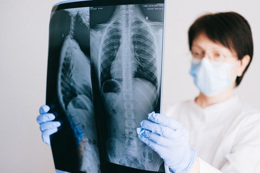
These tasks often formed a pipeline. A lung-nodule system might isolate the lungs, propose small rounded regions, measure each region’s shape and surroundings, then reject candidates that looked more like vessels. If the first step excluded a true nodule, the classifier would never see it. A strong result for the final component could not undo that upstream miss.
Why the pipeline mattered
Preparation and candidate generation
Scans first had to be made reasonably comparable. Depending on the task, preparation might involve intensity normalization, noise reduction, extracting the breast region from a mammogram or correcting slow intensity variation in MRI. Registration mattered in studies comparing images over time: a slight change in patient position could otherwise look like anatomical change.
Candidate generation tended to favor sensitivity. Its job was to retain most true findings, even at the cost of many false alarms. Researchers tried thresholding, filters sensitive to particular shapes, edge analysis and connected-region methods. There was a practical reason to narrow the search early: running a complex classifier at every possible location in a volumetric scan was expensive on the computing hardware of the period.
Features and learned decisions
Once a system had candidates, it turned them into numerical descriptions: size, compactness, boundary irregularity, texture or intensity relative to nearby tissue. A roughly spherical shape might support a lung-nodule hypothesis; a tubular pattern continuing across slices might point to a vessel. Neither observation settled the question alone.
Classifiers such as neural networks and support vector machines combined these measurements into learned decisions. Neural networks appeared in 2000s research, but that did not necessarily mean an end-to-end model trained on whole image archives. Researchers often chose and engineered the features themselves. The blog’s account of how machine learning changed image analysis in the mid-2000s gives more context for why feature design remained central as learned classifiers became common.
Learning offered a way to combine several weak clues where a fixed image-processing rule might falter as scanner noise, tissue density or lesion appearance changed. But the resulting decision boundary still depended on which examples were chosen and how they were labeled.
Different images, different kinds of evidence
In mammography, researchers often looked for masses or clusters of microcalcifications. Assessing a mass meant examining its shape and margins amid overlapping tissue. Finding tiny calcifications called for sensitivity to small bright structures without treating every artifact as disease. Computer-aided detection marks directed a reader’s attention to possible findings; they were not interpretations of the complete examination.
Chest CT offered a different trade-off. Its three-dimensional data let researchers check whether a candidate continued across adjacent slices, but also created many more locations to search. Slice thickness and reconstruction settings could change the appearance of small structures. A detector that worked on one collection might prove unreliable on another.
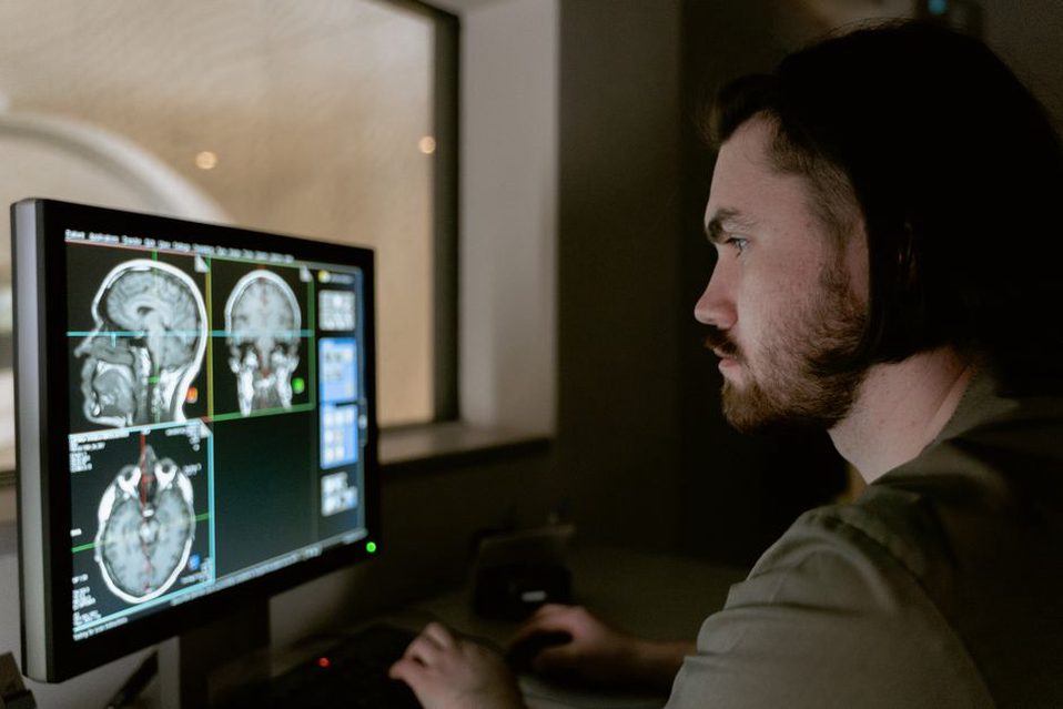
Brain MRI research often focused on segmenting tissues, tumors or anatomical structures. Even expert annotators could disagree about a boundary, and a contour that looked plausible might yield a volume different from a clinician’s reference tracing. Retinal photographs posed other difficulties: changing illumination and camera field could interfere with locating vessels or lesions. “Medical image AI” described a set of specialized research problems, not a single general visual skill.
How researchers measured progress
A headline accuracy figure could hide the trade-off that mattered most. A system might classify numerous normal regions correctly and still miss findings of clinical interest. Researchers therefore used measures suited to the task, including sensitivity for lesion detection, false positives per image or scan, and overlap or boundary measures for segmentation.
Detection studies often plotted sensitivity against the average number of false-positive marks per examination. The trade-off was tangible: more marks might catch more lesions, but someone would have to review them. For segmentation, agreement with a reference outline was informative, though the importance of a small boundary difference depended on the structure being measured and why it was being measured.
How researchers separated training and test data mattered, too. Several slices from one patient did not amount to several independent patients. If related images appeared in both sets, familiar anatomy or acquisition characteristics could make a model seem more general than it was. Testing on separate patients—and preferably on data from another institution—posed a tougher challenge. Reference labels were not all equivalent, either: pathology, follow-up findings and expert image annotations provided different kinds of evidence. An expert’s mark was not always a definitive diagnosis.
What historical results can and cannot establish
Laboratory studies showed that algorithms could detect measurable patterns in medical images. They did not, by themselves, show better patient outcomes. A retrospective study could test whether a detector found annotated nodules, but not whether its use changed care. That required attention to the reading workflow: when marks appeared, whether readers trusted them and what extra false alarms did to interpretation.
When reading an older CT nodule paper, the evaluation design may tell you more than the classifier’s name. Are results counted per lesion or per patient? Are false positives reported per scan? Were test patients kept separate from those used to tune the system? Those details define what the reported detection rate actually means.