
An 8-bit JPEG could look almost unchanged to a person and still produce a different edge map after compression. Blocking changed local intensity differences; smoothing erased weak boundaries; a small threshold adjustment could join regions that had been separate. In a 2000s vision system, later stages often depended on exactly the pixels earlier stages passed along. To understand those systems, it helps to look beneath the recognizer, at signal processing, measurement, optimization, and camera geometry.
Those foundations predated the decade. Fourier analysis, mathematical morphology, statistical estimation, and projective geometry had developed over many years. What changed in the 2000s was the range of images and tasks researchers could tackle: digital cameras became commonplace, scanned archives grew, medical imaging supplied volumetric data, and faster computers made demanding methods more practical. The resulting systems were not a single technology. Each combined choices about sampling, cleaning, representing, and evaluating images.
An image was a measured signal, not a clean grid
The familiar pixel grid hides how an image was made. Light passed through optics, reached a sensor, was integrated over an exposure, sampled at discrete locations, and converted to stored values. Scanners and medical instruments had different acquisition chains, but the same caution applied: recorded intensities were measurements affected by noise, resolution, and device settings, not direct labels for objects.
That signal-processing view helps explain why filtering mattered. A Gaussian blur reduced fine-scale variation by averaging nearby values, giving more weight to those near the center. It could suppress noise before edge detection, but it could also erase a thin line or merge adjacent structures. Sharpening made some boundaries clearer while amplifying noise. A median filter, which replaces a value with the median of its neighborhood, handled isolated bright or dark pixels differently from a linear average. The choice depended on both the unwanted variation and the features an application needed to keep.
Scale changed what counted as a feature
An edge visible at one resolution might disappear after downsampling. Texture that looked irregular close up might form a stable pattern farther away. Scale-space methods examined versions of an image smoothed to different degrees. Gaussian smoothing offered a systematic progression from fine to coarse structure; difference-of-Gaussians calculations could identify locations that stood out against their surroundings across scales.
This gave researchers a way to ask whether a feature survived a change in viewing distance. A character stroke and a page margin occupied very different scales, as did a tiny lesion and the outline of an organ. A single fixed-size neighborhood could not describe both reliably.

Local derivatives connected pixels to structure
Edges were often estimated from spatial derivatives: how rapidly intensity changed across neighboring pixels. Gradient magnitude indicated the strength of a change; gradient direction gave its orientation. Operators such as Sobel approximated these derivatives with small convolution kernels. The Canny detector combined smoothing, gradient estimation, non-maximum suppression, and threshold-based linking to produce thin, connected boundaries.
Each step addressed a different difficulty. Smoothing limited false responses to noise. Non-maximum suppression reduced thick bands to local peaks. Two thresholds let a strong boundary support a weaker neighboring segment without accepting every weak response. The result was still not an object outline. A shadow, printed character, anatomical boundary, or fold in paper could all generate gradients. Later stages had to supply context.
That distinction mattered when assessing a pipeline. A gain measured only after classification might seem to come from the classifier when steadier edge extraction was responsible. Conversely, an attractive edge map might not help recognition if it preserved the wrong boundaries. Intermediate outputs were diagnostic evidence, not ends in themselves.
Geometry supplied constraints that appearance could not
Computer vision drew on photogrammetry and projective geometry. A camera mapped points in three-dimensional space to positions in a two-dimensional image. Knowing or estimating that mapping helped researchers tell a change in object shape from a change in viewpoint. Calibration also mattered when measurements in an image had to correspond to physical distances.
In stereo imaging, two cameras observed the same scene from different positions. A point’s displacement between views—its disparity—could support a depth estimate when the camera geometry was known. Establishing which pixel or patch in one view matched which in the other was harder. Repeated patterns, untextured walls, reflections, and occlusion all made correspondence ambiguous. Image processing helped compare local neighborhoods and enforce spatial consistency; geometry ruled out implausible matches.
Geometry guided less elaborate tasks, too. Rectifying a photographed page could make text lines approximately horizontal before recognition. Registering medical scans brought corresponding anatomy into a shared coordinate frame before measuring change. Alignment error or downstream measurements could then test the result more meaningfully than whether the image merely looked straighter.
Regions brought set theory into the pixel grid
Many applications needed areas rather than edges: the ink of a character, a cell in a microscope image, or a foreground object. Thresholding was the simplest route, assigning pixels to groups by intensity or color. A global threshold worked when foreground and background were well separated. Uneven illumination, faded paper, and variable tissue contrast called for local decisions or more elaborate segmentation.
Mathematical morphology treated a binary region as a set of pixel locations. Erosion shrank it according to a chosen structuring element; dilation expanded it. Combinations could remove isolated marks or bridge narrow gaps. But the element’s shape and size encoded an assumption about what mattered. A setting that repaired broken text strokes might join neighboring characters. One that removed specks from a microscope image might remove small cells.
Connected-component analysis grouped touching foreground pixels into candidate regions. It helped find character candidates or count segmented objects, but depended on upstream choices about illumination correction, thresholds, and morphology. Converting pixels into sets made measures such as area, perimeter, holes, and adjacency available. It also gave early errors another route through the pipeline.
Probability and optimization handled ambiguity
A hard threshold made a decision at each pixel even when the evidence was uncertain. Statistical methods could instead weigh competing explanations: a pixel might fit a foreground model better than a background model while its neighbors favored the opposite assignment. Bayesian reasoning offered a framework for combining observations with prior assumptions. Energy-minimization methods expressed some versions of the problem as a balance between agreement with the image and constraints such as smoothness.
Graph-cut methods represented possible region assignments in a graph, with costs reflecting image evidence and relationships between neighboring pixels. Under suitable formulations, a minimum cut gave an efficient solution. Active contours took another approach: a curve moved in response to image evidence and constraints on its shape. Neither removed the need for judgment. Too much smoothness could erase narrow structures; too little could leave a boundary fragmented by noise. An automatic segmentation still reflected assumptions about plausible shapes.
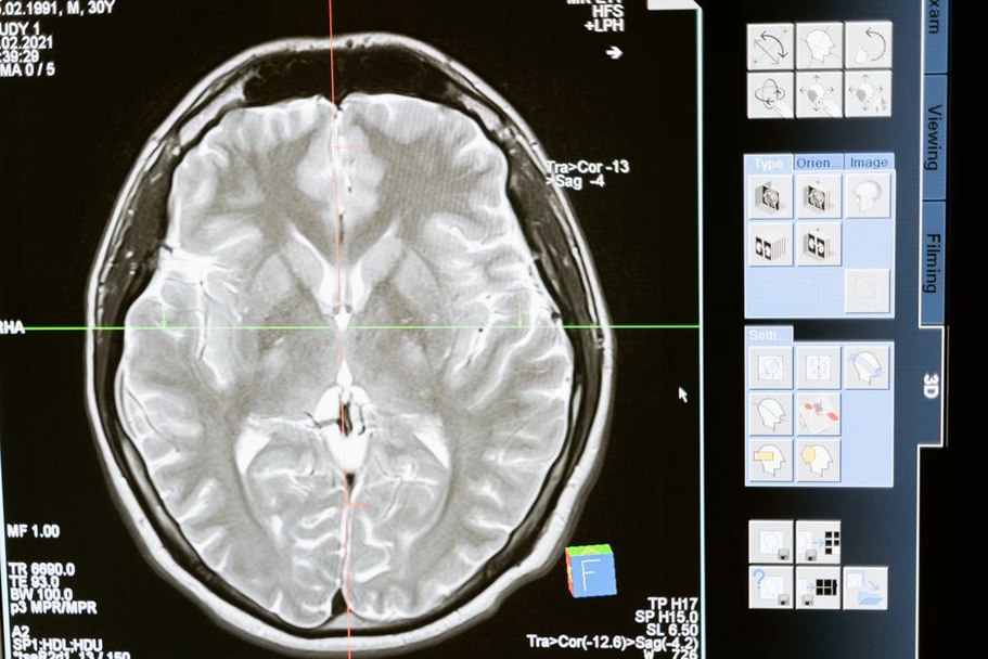
Those assumptions were especially apparent in clinical and scientific images. A boundary might be visually uncertain because tissue contrast was weak, not because the algorithm was poorly implemented. Comparing a computed region with an expert annotation helped, but disagreement between experts could also expose ambiguity in the task. An overlap score alone would not show whether missed pixels lay on a clinically significant boundary or in a less consequential area.
Feature descriptors translated images into comparisons
After finding candidate locations or regions, a system needed numbers it could compare. Raw pixel patches were sensitive to shifts, scale, lighting, and rotation. Hand-designed descriptors tried to retain useful information while reducing some of that sensitivity.
Histograms of oriented gradients summarized the distribution of edge directions in local cells, capturing aspects of shape without requiring exact pixel matches. SIFT described local gradient patterns around keypoints selected across scale and used orientation handling to improve tolerance of rotation. Neither made every variation harmless: a severe viewpoint change, blur, or weak texture could still defeat a match. These descriptors provided a carefully engineered connection between signal processing and recognition.
It helps to separate three tasks often folded into the word “recognition”:
- Detection located a candidate object, region, or keypoint in an image.
- Description converted its appearance or shape into measurements that could be compared.
- Decision matched, classified, or rejected the candidate using a rule learned from data or specified by the application.
A failure in one stage did not mean the others were unsound. If a keypoint detector chose different locations in two views of the same object, a good descriptor could not rescue the match. If detection was stable but the descriptor changed with illumination, the decision stage received inconsistent evidence. This matters when reading results from the period: the same classifier could perform differently with different preprocessing and descriptors.
Computation and data shaped the methods
Researchers in the 2000s had ambitious models, but memory, processor time, and annotated examples limited what they could test. Convolution with small kernels was efficient and reusable. Image pyramids let detectors search across sizes without redesigning their core operation. Integral images sped up sums over rectangular regions, helping methods that evaluated many candidate windows. Such choices could determine whether a technique processed a collection of scans overnight or ran near real time on video.
Training data posed another limit. A model tuned on clean, evenly lit images might fail with a different scanner or camera. Researchers used normalization, augmentation, and separation of training and test material, though practices varied. To judge a comparison, readers needed to know whether methods received the same inputs and whether test images resembled the conditions the system would face. Near-duplicate frames from one video, for example, could make a test split appear more independent than it was.
Benchmark scores were only part of the historical record. Runtime, image resolution, annotation rules, and the handling of failed detections all affected what a result meant. One paper might optimize boundary overlap; another might prioritize thin structures. Neither score explained that trade-off without the task definition.
The boundaries between techniques were productive
The most capable pipelines crossed disciplinary lines. Signal processing reduced acquisition noise; geometry narrowed the search for correspondences; morphology cleaned candidate regions; statistical models resolved uncertain labels; descriptors supplied measurements to a matcher or classifier. Order mattered. Heavy blurring before a search for small keypoints could erase the evidence needed for matching. Segmenting before correcting uneven illumination could make a threshold respond to lighting rather than the object.
Consider a digitized page with faint type and a dark crease. One defensible workflow would estimate the slowly varying background, examine text at a scale suited to its strokes, and then form candidate character regions. The crease might need separate treatment: it is broad and dark, not shaped like a letter. The useful check is not simply whether the page looks cleaner. Does the faint character beside the crease remain connected and distinct?